Note
Go to the end to download the full example code.
3.1 probablistic NN (Disinfection Efficiency)
This file shows how to capture aleoteric uncertainty in a neural network for modeling microbial disinfection efficiency (%) data.
# First we import all the required libaries/functions

import os

import numpy as np  # for array processing

import pandas as pd

import matplotlib.pyplot as plt  # for plotting

from easy_mpl import plot  # plotting functions

from SeqMetrics import RegressionMetrics  # to calculate performance metrics

from ai4water.utils import TrainTestSplit  # for splitting the data into training and test sets
from ai4water.utils.utils import get_version_info

# some helper functions
from utils import read_data, BayesModel, SAVE
from utils import set_rcParams, residual_plot, regression_plot
print version of libraries being used.
for lib,ver in get_version_info().items():
    print(lib, ver)
python 3.9.20 (main, Nov  5 2024, 16:07:55)
[GCC 11.4.0]
os posix
ai4water 1.07
easy_mpl 0.21.4
SeqMetrics 2.0.0
tensorflow 2.10.1
keras.api._v2.keras 2.10.0
numpy 1.21.6
pandas 1.5.3
matplotlib 3.7.1
h5py 3.13.0
sklearn 1.3.1
seaborn 0.13.2
setting global values for plotting
set_rcParams()
Define loss function
def negative_loglikelihood(targets, estimated_distribution):
    return -estimated_distribution.log_prob(targets)
prepare data
data = read_data()

input_features = data.columns.tolist()[0:-1]
output_features = data.columns.tolist()[-1:]

print(input_features)
['Time (min)', 'Ini. CC', 'Sonic. PD', 'h20 Conc.', 'Volume (mL)', 'Solution pH']
print(output_features)
['Efficiency']
split data into training and test sets We set the seed for reproducibility. This will ensure that on very run, the data is splitted in exactly the same way.
TrainX, TestX, TrainY, TestY = TrainTestSplit(seed=313).split_by_random(
    data[input_features],
    data[output_features]
)

# printing the shape of training and test arrays
print(TrainX.shape, TestX.shape, TrainY.shape, TestY.shape)
(219, 6) (95, 6) (219, 1) (95, 1)
hyperparameters
Following hyperparameters have been optimized for the given dataset.
The hidden layers will consist of four fully connected layers and each layer will consist of 32 neurrons.
hidden_units = [32, 32, 32, 32]
learning_rate = 0.0043944
activation = "elu"
train_size = len(TrainX)

num_epochs = 1000
batch_size = 40
uncertainty_type = "aleoteric"
Model Building and training
model = BayesModel(
    model = {"layers": dict(hidden_units=hidden_units,
                            train_size=train_size,
                            activation=activation,
                            uncertainty_type=uncertainty_type,
                            )},
    batch_size=batch_size,
    epochs=num_epochs,
    lr=learning_rate,
    input_features=input_features,
    output_features=output_features,
    category= "DL",
    optimizer="RMSprop",
    loss = negative_loglikelihood,
    #wandb_config=dict(project="flowcam", entity="atherabbas", monitor="val_loss")
)

# resetting global seed for reproducibility
model.reset_global_seed(313)
            building DL model for
            regression problem using layers
Model: "model"
_________________________________________________________________
 Layer (type)                Output Shape              Param #
=================================================================
 input_1 (InputLayer)        [(None, 6)]               0

 batch_normalization (BatchN  (None, 6)                24
 ormalization)

 dense (Dense)               (None, 32)                224

 dense_1 (Dense)             (None, 32)                1056

 dense_2 (Dense)             (None, 32)                1056

 dense_3 (Dense)             (None, 32)                1056

 dense_4 (Dense)             (None, 2)                 66

 independent_normal (Indepen  ((None, 1),              0
 dentNormal)                  (None, 1))

=================================================================
Total params: 3,482
Trainable params: 3,470
Non-trainable params: 12
_________________________________________________________________
dot plot of model could not be plotted due to You must install pydot (`pip install pydot`) and install graphviz (see instructions at https://graphviz.gitlab.io/download/) for plot_model to work.
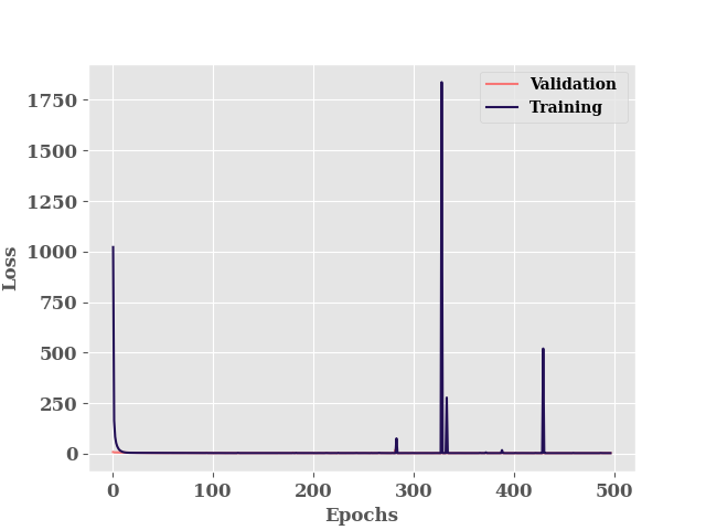
model training
We provide the test data (x,y pairs for test set) as validation_data. This
data will be used for early stopping.
h = model.fit(
    x=TrainX.values.astype(np.float32),
    y=TrainY.values.astype(np.float32),
    validation_data=(TestX.values.astype(np.float32), TestY.values.astype(np.float32)),
    verbose=0
)
********** Successfully loaded weights from weights_396_3.04718.hdf5 file **********
Since our model is probabalistic, we can see that it gives different prediction even though we make prediction on same input data
for i in range(5):
    print(model.predict(TestX[0:2], verbose=False).reshape(-1,))
[43.098385 38.313217]
[ 4.6727104 54.98606  ]
[26.041084 65.09413 ]
[38.01809  39.603497]
[17.294708 45.028538]
Prediction on Training data
If we call the model, the output is the learned distribution.
train_dist = model._model(TrainX)

print(type(train_dist))
<class 'tensorflow_probability.python.layers.internal.distribution_tensor_coercible._TensorCoercible'>
train_mean = train_dist.mean().numpy().reshape(-1,)
train_std = train_dist.stddev().numpy().reshape(-1, )
pd.DataFrame(
np.column_stack([train_mean, TrainY.values]),
columns=['true', 'prediction']
).to_csv(os.path.join(model.path, 'train.csv'), index=False)
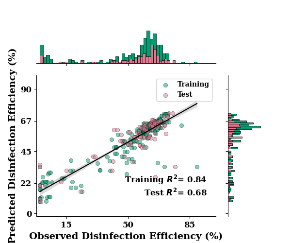
metrics = RegressionMetrics(TrainY.values, train_mean)
print(f"R2: {metrics.r2()}")
print(f"R2 Score: {metrics.r2_score()}")
print(f"RMSE Score: {metrics.rmse()}")
print(f"MAE: {metrics.mae()}")
R2: 0.836968806030221
R2 Score: 0.8152239921144592
RMSE Score: 9.297222541448338
MAE: 5.5407476271
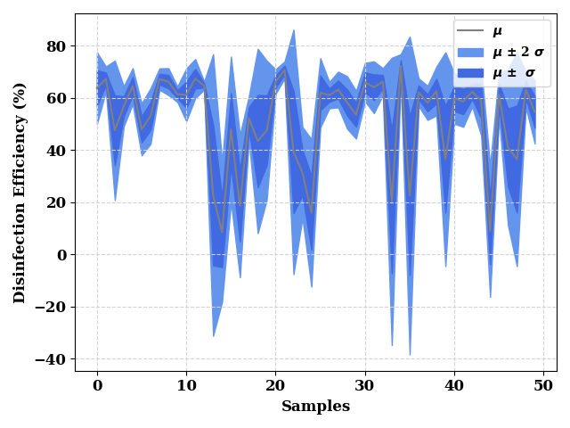
st, en = 0, 50  # draw CI for first 50 samples only

_, ax = plt.subplots()
ax.grid(visible=True, ls='--', color='lightgrey')
ax = plot(train_mean[st:en], show=False, color="grey", label="$\mu$",
          ax_kws=dict(ylabel="Disinfection Efficiency (%)", xlabel="Samples",
                      ylabel_kws={"fontsize": 12, 'weight': 'bold'},
                      xlabel_kws={"fontsize": 12, 'weight': 'bold'}),
          ax=ax,
          )

ax.fill_between(np.arange(len(train_std[st:en])),
                train_mean[st:en] - (2* train_std[st:en]),
                train_mean[st:en] + (2* train_std[st:en]),
                color="cornflowerblue",
                label="$\mu$ $\u00B1$ 2 $\sigma$"
                )
ax.fill_between(np.arange(len(train_std[st:en])),
                train_mean[st:en] - train_std[st:en],
                train_mean[st:en] + train_std[st:en],
                color="royalblue",
                label="$\mu$ $\u00B1$  $\sigma$"
                )
ax.grid(visible=True, ls='--', color='lightgrey')
plt.legend()
plt.tight_layout()
plt.show()
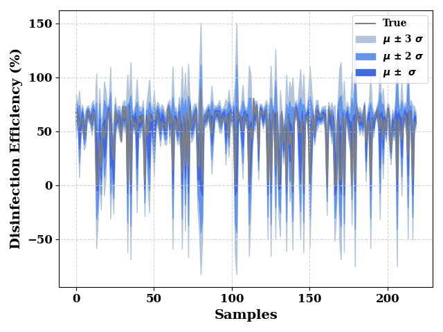
_, ax = plt.subplots()
ax.grid(visible=True, ls='--', color='lightgrey')
ax = plot(TrainY.values, show=False, color="grey", label="True",
          ax_kws=dict(ylabel="Disinfection Efficiency (%)", xlabel="Samples"),
          ax=ax
          )

ax.fill_between(np.arange(len(train_mean)),
                train_mean - (3*train_std),
                train_mean + (3*train_std),
                color="lightsteelblue",
                label="$\mu$ $\u00B1$ 3 $\sigma$",
                )

ax.fill_between(np.arange(len(train_std)),
                train_mean - (2*train_std),
                train_mean + (2*train_std),
                color="cornflowerblue",
                label="$\mu$ $\u00B1$ 2 $\sigma$"
                )
ax.fill_between(np.arange(len(train_std)),
                train_mean - train_std,
                train_mean + train_std,
                color="royalblue",
                label="$\mu$ $\u00B1$  $\sigma$"
                )

plt.legend()
plt.tight_layout()
plt.show()
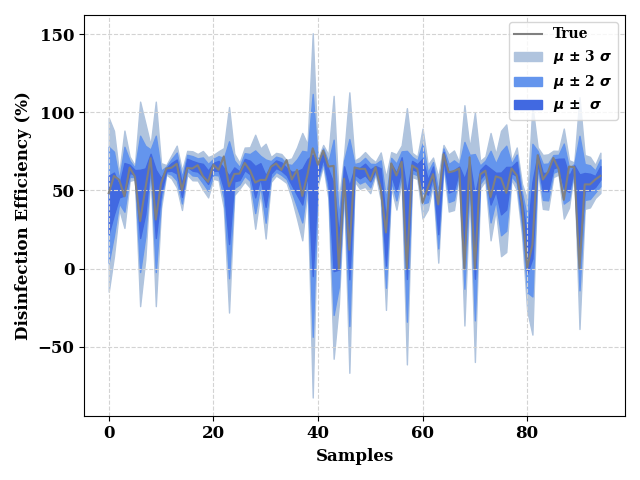
Prediction on Test data
test_dist = model._model(TestX)
test_mean = test_dist.mean().numpy().reshape(-1,)
test_std = test_dist.stddev().numpy().reshape(-1,)

pd.DataFrame(
    np.column_stack([test_mean, TestY.values]),
    columns=['true', 'prediction']
).to_csv(os.path.join(model.path, 'test.csv'), index=False)

metrics = RegressionMetrics(TestY.values, test_mean)
print(f"R2: {metrics.r2()}")
print(f"R2 Score: {metrics.r2_score()}")
print(f"RMSE Score: {metrics.rmse()}")
print(f"MAE: {metrics.mae()}")
R2: 0.6806308826527441
R2 Score: 0.6775488562664058
RMSE Score: 10.285320921172987
MAE: 6.21472232619559
_, ax = plt.subplots()
ax.grid(visible=True, ls='--', color='lightgrey')
ax = plot(test_mean, show=False, color="grey", label="$\mu$",
          ax_kws=dict(ylabel="Disinfection Efficiency (%)", xlabel="Samples"),
          ax=ax,
          )

ax.fill_between(np.arange(len(test_mean)),
                test_mean - (3*test_std),
                test_mean + (3*test_std),
                color="lightsteelblue",
                label="$\mu$ $\u00B1$ 3 $\sigma$",

                )

ax.fill_between(np.arange(len(test_mean)),
                test_mean - (2*test_std),
                test_mean + (2*test_std),
                color="cornflowerblue",
                label="$\mu$ $\u00B1$ 2 $\sigma$"
                )
ax.fill_between(np.arange(len(test_mean)),
                test_mean - test_std,
                test_mean + test_std,
                color="royalblue",
                label="$\mu$ $\u00B1$  $\sigma$"
                )
ax.grid(visible=True, ls='--', color='lightgrey')
plt.legend()
plt.tight_layout()
plt.show()
_, ax = plt.subplots()
ax.grid(visible=True, ls='--', color='lightgrey')
ax = plot(TestY.values, show=False, color="grey", label="True",
          ax_kws=dict(ylabel="Disinfection Efficiency (%)", xlabel="Samples",
                      ylabel_kws={"fontsize": 12, 'weight': 'bold'},
                      xlabel_kws={"fontsize": 12, 'weight': 'bold'}),
          ax=ax
          )

ax.fill_between(np.arange(len(test_mean)),
                test_mean - (3*test_std),
                test_mean + (3*test_std),
                color="lightsteelblue",
                label="$\mu$ $\u00B1$ 3 $\sigma$",
                )

ax.fill_between(np.arange(len(test_mean)),
                test_mean - (2*test_std),
                test_mean + (2*test_std),
                color="cornflowerblue",
                label="$\mu$ $\u00B1$ 2 $\sigma$"
                )
ax.fill_between(np.arange(len(test_mean)),
                test_mean - test_std,
                test_mean + test_std,
                color="royalblue",
                label="$\mu$ $\u00B1$  $\sigma$"
                )
ax.grid(visible=True, ls='--', color='lightgrey')
plt.legend()
plt.tight_layout()
plt.show()
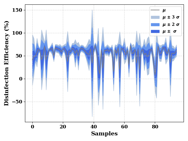
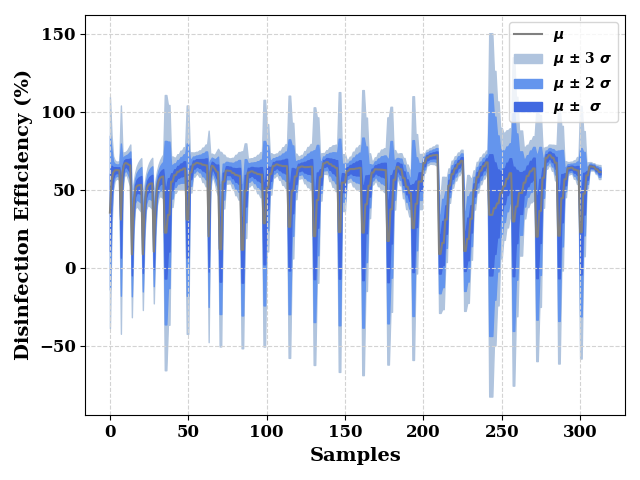
total_dist = model._model(data[input_features])
total_mean = total_dist.mean().numpy().reshape(-1,)
total_std = total_dist.stddev().numpy().reshape(-1,)
_, ax = plt.subplots()
ax.grid(visible=True, ls='--', color='lightgrey')
ax = plot(total_mean, show=False, color="grey", label="$\mu$",
          ax_kws=dict(ylabel="Disinfection Efficiency (%)", xlabel="Samples"),
          ax=ax,
          )

ax.fill_between(np.arange(len(total_mean)),
                total_mean - (3 * total_std),
                total_mean + (3 * total_std),
                color="lightsteelblue",
                label="$\mu$ $\u00B1$ 3 $\sigma$",
                )

ax.fill_between(np.arange(len(total_mean)),
                total_mean - (2 * total_std),
                total_mean + (2 * total_std),
                color="cornflowerblue",
                label="$\mu$ $\u00B1$ 2 $\sigma$"
                )
ax.fill_between(np.arange(len(total_mean)),
                total_mean - total_std,
                total_mean + total_std,
                color="royalblue",
                label="$\mu$ $\u00B1$  $\sigma$"
                )
ax.grid(visible=True, ls='--', color='lightgrey')
plt.legend()
plt.tight_layout()
plt.show()
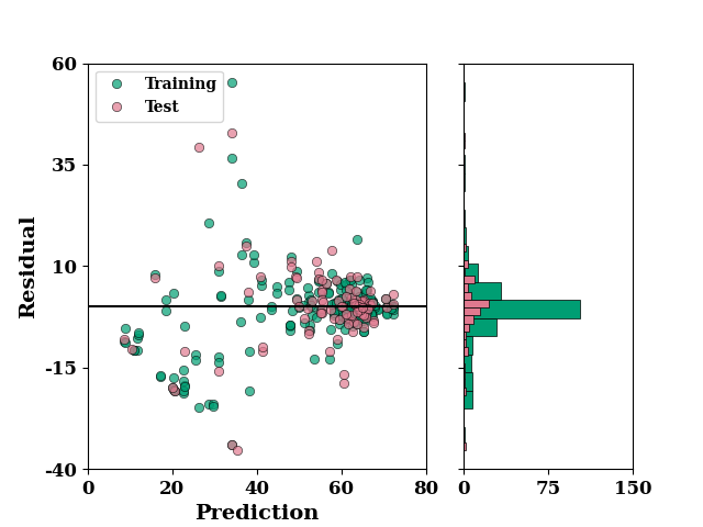
set_rcParams()

residual_plot(
    TrainY.values,
    train_mean,
    TestY.values,
    test_mean,
)
if SAVE:
    plt.savefig("results/figures/residue_aleoteric_eff", dpi=600, bbox_inches="tight")
plt.show()
ax = regression_plot(
    TrainY.values, train_mean,
    TestY.values, test_mean,
    label="Disinfection Efficiency (%)"
)
ax.set_xlim([-2, 100])
ax.set_ylim([-2, 100])
if SAVE:
    plt.savefig("results/figures/reg_aleot_eff", dpi=600, bbox_inches="tight")
plt.show()
*c* argument looks like a single numeric RGB or RGBA sequence, which should be avoided as value-mapping will have precedence in case its length matches with *x* & *y*. Please use the *color* keyword-argument or provide a 2D array with a single row if you intend to specify the same RGB or RGBA value for all points.
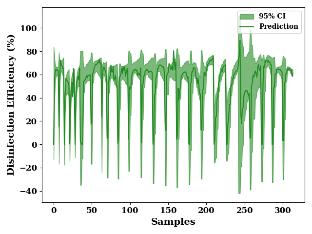
plot 95 % confidence interval
total_upper = total_mean + (1.96 * total_std)
total_lower = total_mean - (1.96 * total_std)

_, ax = plt.subplots()
ax.fill_between(np.arange(len(total_lower)),
                total_upper, total_lower,
                label="95% CI",
                alpha=0.6, color='forestgreen')
_ = plot(data[output_features].values,
         color="forestgreen", label="Prediction",
          ax=ax, show=False)
ax.set_xlabel("Samples")
ax.set_ylabel("Disinfection Efficiency (%)")
if SAVE:
    plt.savefig("results/figures/ci_95_aleot_eff", dpi=600, bbox_inches="tight")
plt.tight_layout()
plt.show()
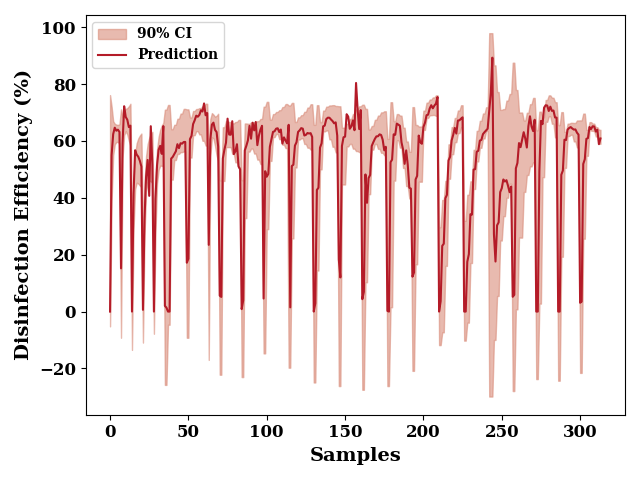
plot the 90% confidence interval
total_upper = total_mean + (1.645 * total_std)
total_lower = total_mean - (1.645 * total_std)

_, ax = plt.subplots()
ax.fill_between(np.arange(len(total_lower)),
                total_upper, total_lower,
                label="90% CI",
                alpha=0.6,
                color=np.array([217, 140, 122])/255)
_ = plot(data[output_features].values, color=np.array([180, 27, 40])/255,
         label="Prediction",
          ax=ax, show=False)
ax.set_xlabel("Samples")
ax.set_ylabel("Disinfection Efficiency (%)")
if SAVE:
    plt.savefig("results/figures/ci_90_aleot_eff", dpi=600, bbox_inches="tight")
plt.tight_layout()
plt.show()
Total running time of the script: (0 minutes 16.765 seconds)