Note
Go to the end to download the full example code.
3.2 Probablistic NN for Area
This file shows how to capture aleoteric uncertainty in a neural network for modeling microbial cell area data. All the code in this file is exactly similar as in previous file for prediction of cell count with the difference that here we are predicting a different target.
import os

import numpy as np

import pandas as pd

import matplotlib.pyplot as plt

from easy_mpl import plot

from SeqMetrics import RegressionMetrics

from ai4water.utils import TrainTestSplit

from utils import SAVE
from utils import read_data, BayesModel, version_info
from utils import set_rcParams, regression_plot, residual_plot
for lib,ver in version_info().items():
    print(lib, ver)
python 3.9.20 (main, Nov  5 2024, 16:07:55)
[GCC 11.4.0]
os posix
ai4water 1.07
easy_mpl 0.21.4
SeqMetrics 2.0.0
tensorflow 2.10.1
keras.api._v2.keras 2.10.0
numpy 1.21.6
pandas 1.5.3
matplotlib 3.7.1
h5py 3.13.0
sklearn 1.3.1
seaborn 0.13.2
ngboost 0.4.1
shap 0.41.0
set_rcParams()

def negative_loglikelihood(targets, estimated_distribution):
    return -estimated_distribution.log_prob(targets)
data = read_data(target='Area (ABD) Mean')

input_features = data.columns.tolist()[0:-1]
output_features = data.columns.tolist()[-1:]

print(input_features)
['Time (min)', 'Ini. CC', 'Sonic. PD', 'h20 Conc.', 'Volume (mL)', 'Solution pH']
TrainX, TestX, TrainY, TestY = TrainTestSplit(seed=313).split_by_random(
    data[input_features],
    data[output_features]
)
print(TrainX.shape, TestX.shape, TrainY.shape, TestY.shape)
(219, 6) (95, 6) (219, 1) (95, 1)
hyperparameters
hidden_units = [12, 12, 12]
learning_rate = 0.004684
activation = "relu"
train_size = len(TrainX)

num_epochs = 1200
batch_size = 16
uncertainty_type = "aleoteric"
model = BayesModel(
    model = {"layers": dict(hidden_units=hidden_units,
                            train_size=train_size,
                            activation=activation,
                            uncertainty_type=uncertainty_type,
                            )},
    batch_size=batch_size,
    epochs=num_epochs,
    lr=learning_rate,
    input_features=input_features,
    output_features=output_features,
    category= "DL",
    optimizer="RMSprop",
    loss = negative_loglikelihood,
    #wandb_config=dict(project="flowcam", entity="atherabbas", monitor="val_loss")
)
            building DL model for
            regression problem using layers
Model: "model"
_________________________________________________________________
 Layer (type)                Output Shape              Param #
=================================================================
 input_1 (InputLayer)        [(None, 6)]               0

 batch_normalization (BatchN  (None, 6)                24
 ormalization)

 dense (Dense)               (None, 12)                84

 dense_1 (Dense)             (None, 12)                156

 dense_2 (Dense)             (None, 12)                156

 dense_3 (Dense)             (None, 2)                 26

 independent_normal (Indepen  ((None, 1),              0
 dentNormal)                  (None, 1))

=================================================================
Total params: 446
Trainable params: 434
Non-trainable params: 12
_________________________________________________________________
dot plot of model could not be plotted due to You must install pydot (`pip install pydot`) and install graphviz (see instructions at https://graphviz.gitlab.io/download/) for plot_model to work.
h = model.fit(
    x=TrainX.values.astype(np.float32),
      y=TrainY.values.astype(np.float32),
      validation_data=(TestX.values.astype(np.float32), TestY.values.astype(np.float32)),
      verbose=0
              )
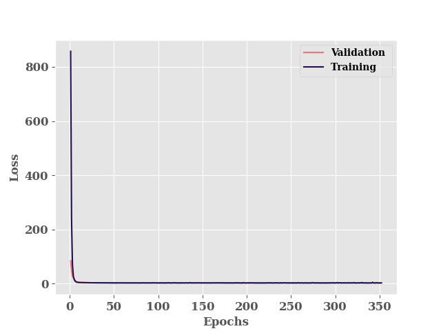
********** Successfully loaded weights from weights_252_2.70156.hdf5 file **********
Since our model is probabalistic, we can see that it gives different prediction even though we make prediction on same input data
for i in range(5):
    print(model.predict(TestX[0:2], verbose=False).reshape(-1,))
[47.419796 30.973263]
[21.256348 42.301834]
[35.80574 49.16989]
[43.9607  31.84996]
[29.850471 35.53607 ]
Prediction on Training data
train_dist = model._model(TrainX)

print(type(train_dist))
<class 'tensorflow_probability.python.layers.internal.distribution_tensor_coercible._TensorCoercible'>
train_mean = train_dist.mean().numpy().reshape(-1,)
train_std = train_dist.stddev().numpy().reshape(-1, )

pd.DataFrame(
    np.column_stack([train_mean, TrainY.values]),
    columns=['true', 'prediction']
).to_csv(os.path.join(model.path, 'train.csv'))

metrics = RegressionMetrics(TrainY.values, train_mean)
print(f"R2: {metrics.r2()}")
print(f"R2 Score: {metrics.r2_score()}")
print(f"RMSE Score: {metrics.rmse()}")
print(f"MAE: {metrics.mae()}")
R2: 0.7942434283409977
R2 Score: 0.7455919650341503
RMSE Score: 8.987235357441008
MAE: 4.693869665485539
st, en = 0, 50
ax = plot(train_mean[st:en], show=False, color="grey", label="$\mu$",
          ax_kws=dict(ylabel="Area (Mean)", xlabel="Samples"),
          )

ax.fill_between(np.arange(len(train_std[st:en])),
                train_mean[st:en] - (2* train_std[st:en]),
                train_mean[st:en] + (2* train_std[st:en]),
                color="cornflowerblue",
                label="$\mu$ $\u00B1$ 2 $\sigma$"
                )
ax.fill_between(np.arange(len(train_std[st:en])),
                train_mean[st:en] - train_std[st:en],
                train_mean[st:en] + train_std[st:en],
                color="royalblue",
                label="$\mu$ $\u00B1$  $\sigma$"
                )
ax.grid(visible=True, ls='--', color='lightgrey')
plt.legend()
plt.tight_layout()
plt.show()

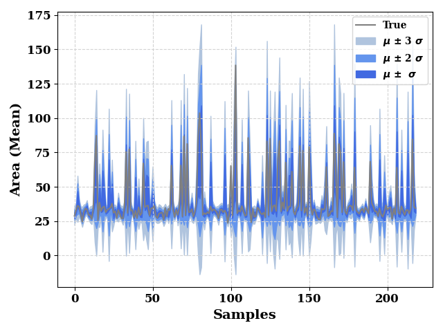
ax = plot(TrainY.values, show=False, color="grey", label="True",
          ax_kws=dict(ylabel="Area (Mean)", xlabel="Samples"),
          )

ax.fill_between(np.arange(len(train_mean)),
                train_mean - (3*train_std),
                train_mean + (3*train_std),
                color="lightsteelblue",
                label="$\mu$ $\u00B1$ 3 $\sigma$",
                )

ax.fill_between(np.arange(len(train_std)),
                train_mean - (2*train_std),
                train_mean + (2*train_std),
                color="cornflowerblue",
                label="$\mu$ $\u00B1$ 2 $\sigma$"
                )
ax.fill_between(np.arange(len(train_std)),
                train_mean - train_std,
                train_mean + train_std,
                color="royalblue",
                label="$\mu$ $\u00B1$  $\sigma$"
                )
ax.grid(visible=True, ls='--', color='lightgrey')
plt.legend()
plt.tight_layout()
plt.show()
Prediction on Test data
test_dist = model._model(TestX)
test_mean = test_dist.mean().numpy().reshape(-1,)
test_std = test_dist.stddev().numpy().reshape(-1,)

pd.DataFrame(
    np.column_stack([test_mean, TestY.values]),
    columns=['true', 'prediction']
).to_csv(os.path.join(model.path, 'test.csv'))

metrics = RegressionMetrics(TestY.values, test_mean)
print(f"R2: {metrics.r2()}")
print(f"R2 Score: {metrics.r2_score()}")
print(f"RMSE Score: {metrics.rmse()}")
print(f"MAE: {metrics.mae()}")
R2: 0.6481352385647595
R2 Score: 0.5497750596253121
RMSE Score: 13.409564004284338
MAE: 5.750466840242086
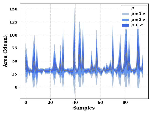
ax = plot(test_mean, show=False, color="grey", label="$\mu$",
          ax_kws=dict(ylabel="Area (Mean)", xlabel="Samples"),
          )

ax.fill_between(np.arange(len(test_mean)),
                test_mean - (3*test_std),
                test_mean + (3*test_std),
                color="lightsteelblue",
                label="$\mu$ $\u00B1$ 3 $\sigma$",

                )

ax.fill_between(np.arange(len(test_mean)),
                test_mean - (2*test_std),
                test_mean + (2*test_std),
                color="cornflowerblue",
                label="$\mu$ $\u00B1$ 2 $\sigma$"
                )
ax.fill_between(np.arange(len(test_mean)),
                test_mean - test_std,
                test_mean + test_std,
                color="royalblue",
                label="$\mu$ $\u00B1$  $\sigma$"
                )
ax.grid(visible=True, ls='--', color='lightgrey')
plt.legend()
plt.tight_layout()
plt.show()
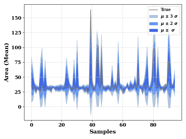
ax = plot(TestY.values, show=False, color="grey", label="True",
          ax_kws=dict(ylabel="Area (Mean)", xlabel="Samples"),
          )

ax.fill_between(np.arange(len(test_mean)),
                test_mean - (3*test_std),
                test_mean + (3*test_std),
                color="lightsteelblue",
                label="$\mu$ $\u00B1$ 3 $\sigma$",
                )

ax.fill_between(np.arange(len(test_mean)),
                test_mean - (2*test_std),
                test_mean + (2*test_std),
                color="cornflowerblue",
                label="$\mu$ $\u00B1$ 2 $\sigma$"
                )
ax.fill_between(np.arange(len(test_mean)),
                test_mean - test_std,
                test_mean + test_std,
                color="royalblue",
                label="$\mu$ $\u00B1$  $\sigma$"
                )
ax.grid(visible=True, ls='--', color='lightgrey')
plt.legend()
plt.tight_layout()
plt.show()
total_dist = model._model(data[input_features])
total_mean = total_dist.mean().numpy().reshape(-1,)
total_std = total_dist.stddev().numpy().reshape(-1,)
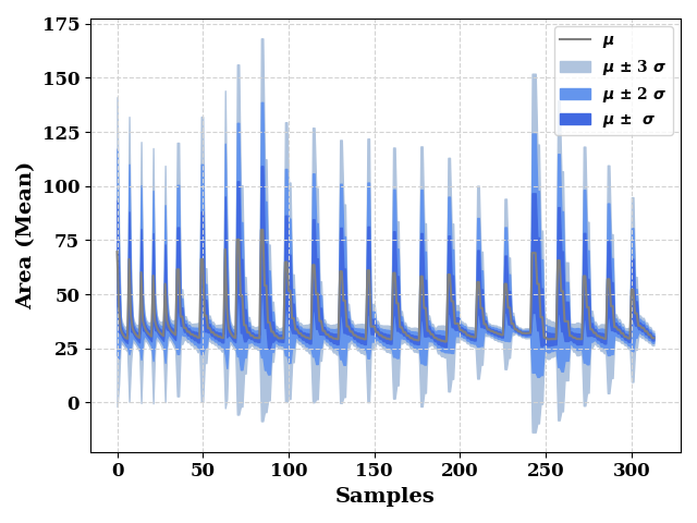
ax = plot(total_mean, show=False, color="grey", label="$\mu$",
ax_kws=dict(ylabel="Area (Mean)", xlabel="Samples"),
)
ax.fill_between(np.arange(len(total_mean)),
total_mean - (3 * total_std),
total_mean + (3 * total_std),
color="lightsteelblue",
label="$\mu$ $\u00B1$ 3 $\sigma$",
)
ax.fill_between(np.arange(len(total_mean)),
total_mean - (2 * total_std),
total_mean + (2 * total_std),
color="cornflowerblue",
label="$\mu$ $\u00B1$ 2 $\sigma$"
)
ax.fill_between(np.arange(len(total_mean)),
total_mean - total_std,
total_mean + total_std,
color="royalblue",
label="$\mu$ $\u00B1$ $\sigma$"
)
ax.grid(visible=True, ls='--', color='lightgrey')
plt.legend()
plt.tight_layout()
plt.show()
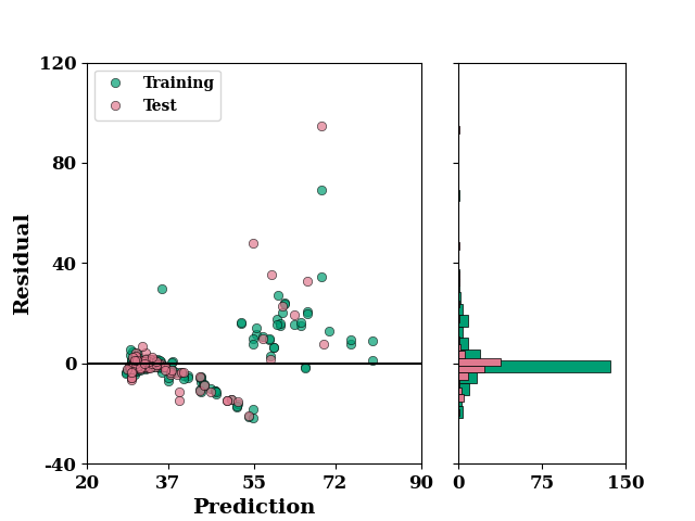
set_rcParams()

residual_plot(
    TrainY.values,
    train_mean,
    TestY.values,
    test_mean,
)
if SAVE:
    plt.savefig("results/figures/residue_aleoteric_area", dpi=600, bbox_inches="tight")
plt.show()
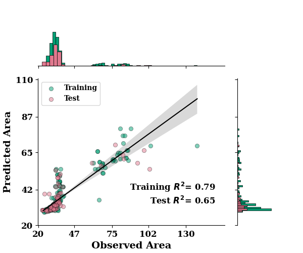
regression_plot(
    TrainY.values, train_mean,
    TestY.values, test_mean,
    max_xtick_val=130,
    max_ytick_val=110,
    min_xtick_val=20,
    min_ytick_val=20,
    label="Area"
)
if SAVE:
     plt.savefig("results/figures/reg_aleot_area", dpi=600, bbox_inches="tight")
plt.show()
*c* argument looks like a single numeric RGB or RGBA sequence, which should be avoided as value-mapping will have precedence in case its length matches with *x* & *y*. Please use the *color* keyword-argument or provide a 2D array with a single row if you intend to specify the same RGB or RGBA value for all points.
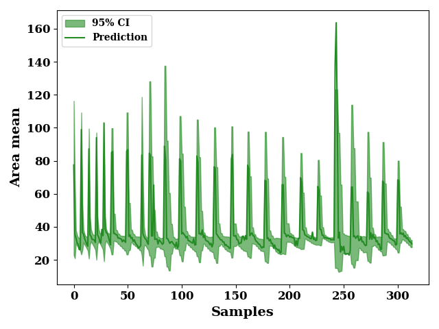
plot 95 % confidence interval
total_upper = total_mean + (1.96 * total_std)
total_lower = total_mean - (1.96 * total_std)

_, ax = plt.subplots()
ax.fill_between(np.arange(len(total_lower)),
                total_upper, total_lower,
                label="95% CI",
                alpha=0.6, color='forestgreen')
_ = plot(data[output_features].values,
         color="forestgreen", label="Prediction",
          ax=ax, show=False)
ax.set_xlabel("Samples")
ax.set_ylabel("Area mean")
if SAVE:
    plt.savefig("results/figures/ci_95_aleot_area", dpi=600, bbox_inches="tight")
plt.tight_layout()
plt.show()
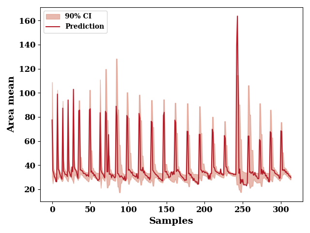
plot the 90% confidence interval
total_upper = total_mean + (1.645 * total_std)
total_lower = total_mean - (1.645 * total_std)

_, ax = plt.subplots()
ax.fill_between(np.arange(len(total_lower)),
                total_upper, total_lower,
                label="90% CI",
                alpha=0.6,
                color=np.array([217, 140, 122])/255)
_ = plot(data[output_features].values, color=np.array([180, 27, 40])/255,
         label="Prediction",
          ax=ax, show=False)
ax.set_xlabel("Samples")
ax.set_ylabel("Area mean")
if SAVE:
    plt.savefig("results/figures/ci_90_aleot_area", dpi=600, bbox_inches="tight")
plt.tight_layout()
plt.show()
Total running time of the script: (0 minutes 15.970 seconds)