4.2 Bayesian NN (Area)

This file shows how to record epistemic uncertainty in a neural network for modeling Cell Area data.

import numpy as np

import matplotlib.pyplot as plt

from easy_mpl import plot

from SeqMetrics import RegressionMetrics

from ai4water.utils import TrainTestSplit
from ai4water.postprocessing import ProcessPredictions

from utils import SAVE, version_info
from utils import read_data, BayesModel
from utils import set_rcParams, regression_plot, residual_plot

for lib, ver in version_info().items():
    print(lib, ver)

python 3.9.20 (main, Nov  5 2024, 16:07:55)
[GCC 11.4.0]
os posix
ai4water 1.07
easy_mpl 0.21.4
SeqMetrics 2.0.0
tensorflow 2.10.1
keras.api._v2.keras 2.10.0
numpy 1.21.6
pandas 1.5.3
matplotlib 3.7.1
h5py 3.13.0
sklearn 1.3.1
seaborn 0.13.2
ngboost 0.4.1
shap 0.41.0

set_rcParams()

data = read_data(target='Area (ABD) Mean')

input_features = data.columns.tolist()[0:-1]
output_features = data.columns.tolist()[-1:]

TrainX, TestX, TrainY, TestY = TrainTestSplit(seed=313).split_by_random(
    data[input_features],
    data[output_features]
)

print(TrainX.shape, TestX.shape, TrainY.shape, TestY.shape)

(219, 6) (95, 6) (219, 1) (95, 1)

hyperparameters

hidden_units = [6, 6]
learning_rate = 0.002632
activation = "relu"
train_size = len(TrainX)

num_epochs = 5000
batch_size = 24
uncertainty_type = "epistemic"

Build model

model = BayesModel(
    model = {"layers": dict(hidden_units = hidden_units,
                            train_size = train_size,
                            activation = activation,
                            uncertainty_type = uncertainty_type
                            )},
    batch_size=batch_size,
    epochs=num_epochs,
    lr=learning_rate,
    input_features=input_features,
    output_features=output_features,
    category= "DL",
    y_transformation="robust",
    optimizer="RMSprop",
    x_transformation=[
        {"method": "log2", "features": ["Time (min)"], "replace_zeros": True},
        {"method": "quantile", "features": ["Ini. CC"]},
        # {"method": "log2", "features": ["sonic_pd"]},
        {"method": "quantile", "features": ["h20 Conc."]},
        {"method": "quantile", "features": ["Volume (mL)"]},
        {"method": "log10", "features": ["Solution pH"]},
    ],
    #wandb_config=dict(project="flowcam", entity="atherabbas", monitor="val_loss")
)

            building DL model for
            regression problem using layers
Model: "model"
_________________________________________________________________
 Layer (type)                Output Shape              Param #
=================================================================
 input_1 (InputLayer)        [(None, 6)]               0

 batch_normalization (BatchN  (None, 6)                24
 ormalization)

 dense_variational (DenseVar  (None, 6)                945
 iational)

 dense_variational_1 (DenseV  (None, 6)                945
 ariational)

 dense (Dense)               (None, 1)                 7

=================================================================
Total params: 1,921
Trainable params: 1,909
Non-trainable params: 12
_________________________________________________________________
dot plot of model could not be plotted due to You must install pydot (`pip install pydot`) and install graphviz (see instructions at https://graphviz.gitlab.io/download/) for plot_model to work.

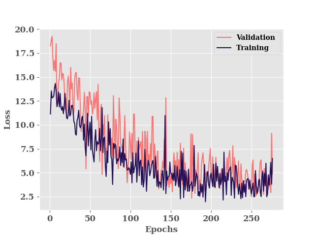
model training

model.fit(TrainX, TrainY, validation_data=(TestX, TestY),
          verbose=0)

********** Successfully loaded weights from weights_176_2.34016.hdf5 file **********

<keras.callbacks.History object at 0x7a6bd2b4f160>

Since the weights of the model are not scaler/constant and they are distributions, everytime we run the forward propagation i.e. we make predictions from the model with same input, we get different output

for i in range(5):
    print(model.predict(
        x=TrainX.iloc[0, :].values.reshape((-1, len(input_features))),
        verbose=0))

[[30.980127]]
[[31.322758]]
[[30.722158]]
[[31.81035]]
[[29.77998]]

training results

Therefore, inorder to get a prediction which we can compare with observed values, we will run the forward propagation n times and take the mean. In our case n is 100.

train_predictions = []
for i in range(100):
    train_predictions.append(model.predict(TrainX, verbose=0))
train_predictions =  np.concatenate(train_predictions, axis=1)

print(train_predictions.shape)

(219, 100)

train_std = np.std(train_predictions, axis=1)
train_mean = np.mean(train_predictions, axis=1)

metrics = RegressionMetrics(TrainY, train_mean)
print(f"R2: {metrics.r2()}")
print(f"R2 Score: {metrics.r2_score()}")
print(f"RMSE Score: {metrics.rmse()}")
print(f"MAE: {metrics.mae()}")

R2: 0.8723001755525356
R2 Score: 0.8626742051955718
RMSE Score: 6.602931076835974
MAE: 3.617493454397541

processor = ProcessPredictions(
    mode="regression", forecast_len=1,
    path=model.path
)

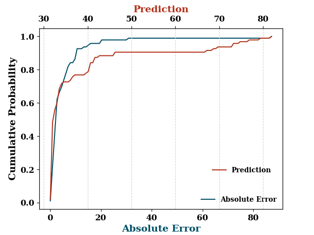
processor.edf_plot(TrainY, train_mean)

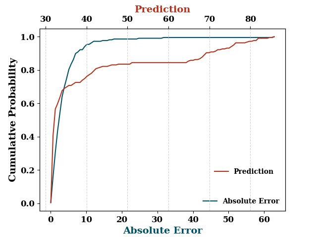
[<Axes: xlabel='Absolute Error', ylabel='Cumulative Probability'>, <Axes: xlabel='Prediction', ylabel='Cumulative Probability'>]

plot(train_mean, '.', label="Prediction Mean", show=False)
plot(TrainY.values, '.', label="True", ax_kws=dict(logy=True))

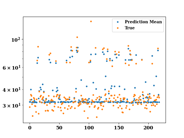
<Axes: >

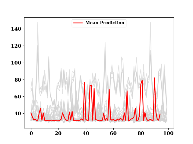
test results

test_predictions = []
for i in range(100):
    test_predictions.append(model.predict(TestX, verbose=0))

test_predictions =  np.concatenate(test_predictions, axis=1)

test_std = np.std(test_predictions, axis=1)
test_mean = np.mean(test_predictions, axis=1)

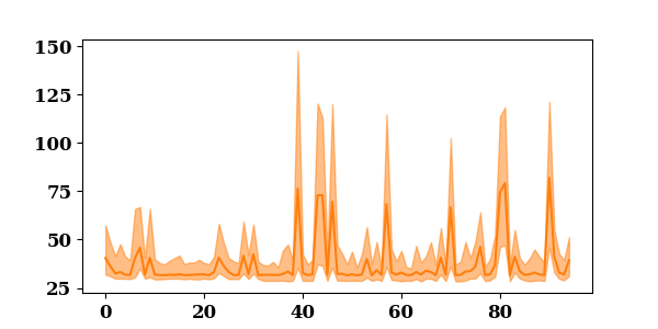
f, ax = plt.subplots()
for i in range(50):

    plot(test_predictions[i], ax=ax, show=False,
         color='lightgray', alpha=0.7)

plot(test_mean, label="Mean Prediction", color="r", lw=2.0, ax=ax)
plt.show()

metrics = RegressionMetrics(TestY, test_mean)
print(f"R2: {metrics.r2()}")
print(f"R2 Score: {metrics.r2_score()}")
print(f"RMSE Score: {metrics.rmse()}")
print(f"MAE: {metrics.mae()}")

R2: 0.7702233216034856
R2 Score: 0.6996612406256144
RMSE Score: 10.952306124898973
MAE: 4.88729334700735

processor.edf_plot(TestY, test_mean)

[<Axes: xlabel='Absolute Error', ylabel='Cumulative Probability'>, <Axes: xlabel='Prediction', ylabel='Cumulative Probability'>]

if model.use_wb:
    model.wb_finish()

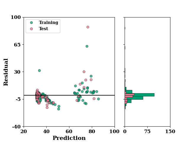
residual_plot(
    TrainY.values,
    train_mean,
    TestY.values,
    test_mean,
)
if SAVE:
    plt.savefig("results/figures/residue_bayes_area", dpi=600, bbox_inches="tight")
plt.show()

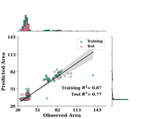
regression_plot(
    TrainY.values, train_mean,
    TestY.values, test_mean,
    min_xtick_val=20, max_xtick_val=145,
    min_ytick_val=20, max_ytick_val=145,
    label="Area"
)
if SAVE:
    plt.savefig("results/figures/reg_bayes_area", dpi=600, bbox_inches="tight")
plt.show()

*c* argument looks like a single numeric RGB or RGBA sequence, which should be avoided as value-mapping will have precedence in case its length matches with *x* & *y*.  Please use the *color* keyword-argument or provide a 2D array with a single row if you intend to specify the same RGB or RGBA value for all points.

lower = np.min(test_predictions, axis=1)
upper = np.max(test_predictions, axis=1)
_, ax = plt.subplots(figsize=(6, 3))
ax.fill_between(np.arange(len(lower)), upper, lower, alpha=0.5, color='C1')
p1 = ax.plot(test_mean, color="C1", label="Prediction")
p2 = ax.fill(np.NaN, np.NaN, color="C1", alpha=0.5)
plt.show()